Home | Simulations
Simple Harmonic Oscillator Simulation - Forced Oscillations

General Aim of Simple Harmonic Oscillator Simulation

In the spring constant experiment, you are going to determine the force constant of a spring statically and dynamically using simple harmonic oscillator simulation.

 

Method of Simple Harmonic Oscillator Simulation

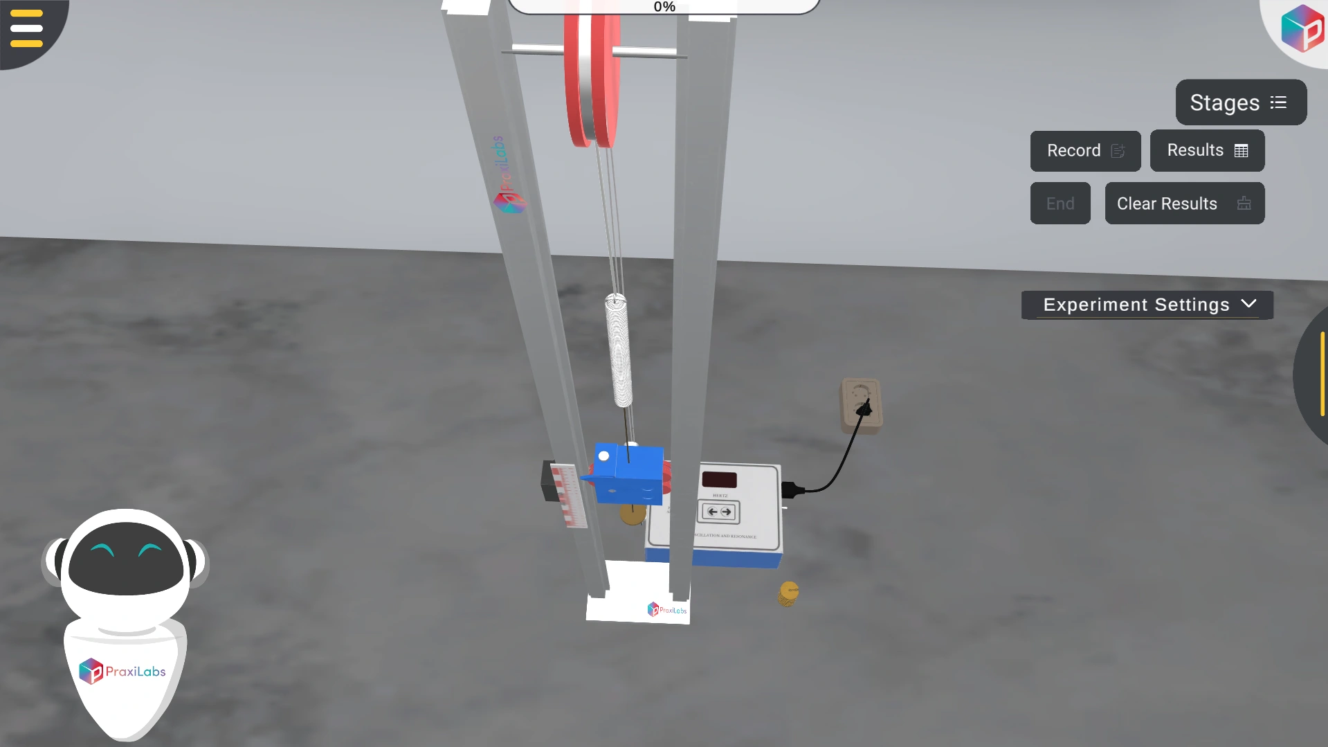
Part (I): Determination of the Force Constant of the Spring Statically by using spring constant simulation In a resonance physics lab, set the apparatus up as shown in Figure (1), making sure the metre rule is parallel to the spring attached to the clamp. Next, in the spring constant virtual lab, measure the natural length of the spring with no force applied to it. With a known mass, apply to the end of the spring and measure the new length during the simple harmonic motion experiment. Figure 1. The experiment setup. Record the data in the table below: Mass (gm) F=mass(kg) * g ∆L=L-L0 Where g is the gravity which is equal to 9.8 m/ s2. Repeat the procedure by increasing the known mass to obtain enough results to formulate a graph. Once all data is collected, use the raw data to create the following graph: Figure 2. Force (N) vs displacement (m) Calculate the value of the spring constant from the equation using a spring constant calculator: F=mg=k ∆L slope=F∆L=k Part (II): Determination of the Force Constant of the Spring Dynamically by using spring constant lab This part deals with the dynamically determined spring constant. By displacing the spring from equilibrium, the system will oscillate. By measuring the mass of the system and its period of oscillation, the value of the spring constant can be deduced. First attach the spring to the clamp stand and attach the mass holder to the spring as shown in the figure below. Then attach the first mass. Wait until the spring stops moving completely, then place the fiducial marker at the very bottom of the mass holder, using the metre ruler to align it perfectly. This represents the center of oscillations and will make it easier to count how many oscillations the mass-spring system has undergone (as shown in figure below). Figure 3. Fiducial marker Then, pull the spring down slightly and let it go so that it is oscillating with a small amplitude and in a straight line. As the bottom of the mass holder passes the fiducial marker, start the stopwatch and count the time taken for it to complete 20 full oscillations (T20). For each different mass record the value of time taken to complete 20 full oscillations in the following table. mass (gm) T20 (sec) T=T2020 (sec) T2 (sec2) Then, plot a graph between T2 in y-axis and mass (kg) in x-axis. Figure 4. Time2(sec2) vs mass (kg) Calculate the value of the spring constant from the equation: T2=42km+42kM k=42slope

Theoretical Background / Context

• Hooke’s law, law of elasticity discovered by the English scientist Robert Hooke in 1660, which states that, for relatively small deformations of an object, the displacement or size of the deformation is directly proportional to the deforming force or load. 
• Under these conditions the object returns to its original shape and size upon removal of the load. 
• Elastic behavior of solids according to Hooke’s law can be explained by the fact that small displacements of their constituent molecules, atoms, or ions from normal positions is also proportional to the force that causes the displacement.
• The deforming force may be applied to a solid by stretching, compressing, squeezing, bending, or twisting. 
• Thus, a metal wire exhibits elastic behavior according to Hooke’s law because the small increase in its length when stretched by an applied force doubles each time the force is doubled. 
• Mathematically, Hooke’s law states that the applied force F equals a constant k times the displacement or change in length x, or F = kx. The value of k depends not only on the kind of elastic material under consideration but also on its dimensions and shape.
• At relatively large values of applied force, the deformation of the elastic material is often larger than expected on the basis of Hooke’s law, even though the material remains elastic and returns to its original shape and size after removal of the force.
•  Hooke’s law describes the elastic properties of materials only in the range in which the force and displacement are proportional.
•  Sometimes Hooke’s law is formulated as F = -kx. In this expression F no longer means the applied force but rather means the equal and oppositely directed restoring force that causes elastic materials to return to their original dimensions.

Principle Of Work

 In the simple harmonic oscillator simulation:

• If an applied force varies linearly with position, the force can be defined as F=ax where a is called the force constant. 
• Once such a physical system where this force exists is with a common helical spring acting on a body. 
• If the spring is stretched or compressed a small distance from its equilibrium position, the spring will exert a force on the body given by Hooke's Law, namely

Fs=-kx       (1)

where Fs is known as the spring force. 

• Here the constant of proportionality, k, is the known as the spring constant, and x is the displacement of the body from its equilibrium position (at x=0 ). 
• The spring constant is an indication of the spring's stiffness. 
• A large value for k indicates that the spring is stiff. A low value for k means the spring is soft.
•  Generally speaking, springs with large k values can balance larger forces than springs with low k values.
• The negative sign in Equation 1 indicates that the direction of Fs is always opposite the direction of the displacement. This implies that the spring force is a restoring force.
•  In other words, the spring force always acts to restore, or return, the body to the equilibrium position regardless of the direction of the displacement, as shown in Figures 5a - 5c.

Figure 5a. When the displacement is to the right (x > 0) the spring force is directed to the left ( Fs< 0).

Figure 5b. When the displacement is to the left (x < 0) the spring force is directed to the right ( Fs> 0).

Figure 5c. In both cases shown in Figures 5a and 5b, the effect of the spring force is to return the system to the equilibrium position. At this position,  x= 0 and the spring is unstretched, signifying  Fs= 0.

• When a mass, m, is suspended from a spring and the system is allowed to reach equilibrium, as shown in Figure 6, Newton's Second Law tells us that the magnitude of the spring force equals the weight of the body, Fs=mg. 
• Therefore, if we know the mass of a body at equilibrium, we can determine the spring force acting on the body.

Figure 6. A body of mass, m, is suspended from a spring having a spring constant, k. If the system is in equilibrium the spring force is balanced by the weight of the body.

• Equation 1 applies to springs that are initially unstretched. When the body undergoes an arbitrary displacement from some initial position, 
• xi, to some final position, xf, this equation can be written as

Fs=-kxf-xi=-k∆x        where ∆x is the body's displacement.

• If the body in Figure 7 is displaced from its equilibrium position some maximum distance, A, and then released, it will oscillate about the equilibrium position. 
• The body will move back and forth between the positions x=+A and x=-A. When the mass travels from the maximum displacement x=+A to the minimum displacement x=-A and then back to the position x=+A, we say that the mass has moved through one cycle, or oscillation. 
• In the simple harmonic oscillator simulation, when an oscillating mass (as in the case of a mass bouncing on a spring) experiences a force that is linearly proportional to its displacement but in the opposite direction, the resulting motion is known as simple harmonic motion. 
• This motion is periodic, meaning the displacement, velocity and acceleration all vary sinusoidally. The time required for the body to complete one oscillation is defined as the period, T, and is given by  T=2πmk 

Figure 7. Experiment setup

• Notice the period is dependent only upon the mass of the oscillating body and the spring constant, 
• k. As the stiffness of the spring increases (that is, as k increases), the period decreases which has the effect of increasing the body's average velocity. 
• Conversely, an increase in the body's mass means the period will also increase, thereby requiring more time for the body to move through one oscillation. 
• It should be noted that the period of motion is independent of the amplitude of the oscillations.